III

Non-local Projector Reduction

in

Optimised Pseudopotentials

In this chapter we describe a method to reduce the number of non-local components of a pseudopotential, i.e. the number of different radial pseudopotentials acting on different angular momenta in the spherical Schrödinger equation. The benefit of treating a pseudopotential in this way is significant for large scale ab initio calculations, especially when the non-local part of the pseudopotential is implemented in real-space in the manner of Ref.K.2. Furthermore, when the non-local components of a pseudopotential are expressed in the form proposed by Kleinman and Bylander [Ref.K.1], eliminating some non-local components can sometimes help to improve the accuracy of the pseudopotential because the Kleinman-Bylander form is approximate and can be somewhat ill-behaved on some components in some cases. Some tests will be presented to show these features of the pseudopotentials generated using this Projector (Component) Reduction technique. We will also present a theoretical interpretation of the procedure and its limitations.

III.1. Introduction

The introduction of ab initio norm-conserving pseudopotentials by Hamann, Schluter and Chiang [Ref.H.1] was a significant step in pseudopotential theory. The "norm-conserving" condition assures that the pseudopotentials reproduce the electrostatic interaction between atoms as well as the scattering of the electronic states by the ions. These features make the pseudopotentials extremely accurate and make them important for modern electronic structure calculations. To generate an ab initio pseudopotential, one first finds the all-electron wave functions for an atom : the pseudopotential is then generated by pseudising the l-dependent radial wave functions and then inverting the radial Schrödinger equation, as described in more detail in Chapter I. The resulting pseudopotential is therefore non-local because of its l-dependence. More precisely, due to the construction from all the l-channels, the pseudopotential has the form

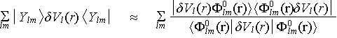
V ^PS = S_lm |Y_lm > V_l (r) <Y_lm | , (1.1)

in which the Y_lm are the spherical harmonics. The pseudopotential in (1.1) is local in the radial coordinate but non-local in the angular coordinates, which is why it is also described as "semi-local". In most cases such a pseudopotential is expressed in terms of a local part V^L(r), which is common for all l, and a non-local part dV_l(r) = V_l(r)-V^L(r) for each angular momentum l, with only dV_l(r) of a few lower l treated explicitly in a calculation. In this way, the V^L(r) is acting as the (pseudo) potential for the rest of the high l states. Since the scattering of very high l is not important (because it corresponds to either high kinetic energy or long interaction distance), as long as a sufficient number of dV_l(r) have been treated explicitly, the choice of the local V^L(r) can be fairly arbitrary without losing the accuracy of the pseudopotential. With this transformation, (1.1) becomes

V ^PS = S_lm |Y_lm> [V ^L(r) + dV_l(r)] <Y_lm| = V ^L(r) + S_lm |Y_lm> dV_l(r) <Y_lm| . (1.2)

Because of the need to perform 2l+1 projections with the Y_lm for each dV_l(r), a non-local (semi-local) pseudopotential is computationally much more expensive than a local one. Much effort has been expended to improve the efficiency, such as the use of the Kleinman-Bylander (KB) [Ref.K.1] form which approximates the double-variable integral as a multiplication of two single-variable ones,

, (1.3)

in which F⁰_lm(r) = j^PS_l(r)Y_lm(q,f), with j^PS_l(r) being the pseudo wavefunction used to create V_l(r). A real-space formalism of KB form has been proposed by King-Smith et al [Ref.K.2] to allow the KB form to be used reliably in real-space, which has the advantage of a much more favourable scaling with respect to the system size when performing non-local operations. Even with those significant improvements, the 2l+1 spherical harmonic projections for each dV_l(r) are still a very heavy numerical burden in ab initio calculations.

On the other hand, the KB form can also be a source of error because it needs to use pseudo wave functions j^PS_l(r) as reference states, as shown in (1.3). It is easy to verify that the KB form is most accurate (in fact it is exact) only when the wave functions of the system under study are identical to the reference wave functions within the region defined by the pseudising radius. This explains why the accuracy of a KB pseudopotential depends on the choice of reference states, which also implies that using a reference state that is quite different from the typical wave function in the application can cause a large error in a KB pseudopotential. Apart from the problem of the reference states, the possibility of KB form being completely wrong, due to so called "ghost states", has also been reported and analysed by Gonze [Ref.G.1].

Various ways have been used to reduce the number of spherical harmonic projection and to improve the accuracy of the KB form. Usually one simply ignores some higher l non-local components that are not occupied in atomic ground states, hoping that the local part can account for them adequately. To avoid the ghost states or to obtain a better accuracy, one can vary the pseudopotential generating parameters such as the electronic configuration, the r_c and the choice of the local potential [Ref.G.1]. One may also include more reference states in the KB form as suggested by Blöchl [Ref.B.1].

The above approaches work in their own right, but lack the advantage of addressing both the question of efficiency and of accuracy together in a single method. In this chapter, we will show that some of the dV_l(r) in (1.2) can be eliminated without loss of the overall accuracy of the pseudopotential. This is achieved by making these dV_l(r) very small so that they are negligible. It is clear that using the least possible number of non-local parts dV_l(r) in a pseudopotential helps not only to avoid the need for the KB form, but also reduces the number of Y_lm projections. The approach of safely eliminate dV_l(r), which we shall call Projector Reduction, is the main issue to be discussed in this chapter.

In the following sections, we will describe the Projector Reduction method and give two examples in Section 2. In Section 3, solid state tests of a projector reduced pseudopotential will be presented, and comparison with a commonly used pseudopotential will be given. The discussion of the simple theory and the limitations of this method forms the Section 4. Finally we will make a brief conclusion in Section 5.

III.2. The Projector Reduction Method and Examples

The Q_c-tuning method described in Chapter II allow us to change the shape of V_l(r) individually. With this ability, we can make two l-dependent potential components V_i(r) and V_j(r) with l = i, j as similar as possible. Once this is achieved, and knowing that the local potential V ^L (r) can be arbitrarily chosen, we simply construct the V ^L (r) from a weighted average of V_i(r) and V_j(r), i.e.

. (2.1)

This makes the non-local potential components

and (2.2)

extremely small because V_i(r)-V_j(r) is small, and therefore both dV_i(r) and dV_j(r) can hopefully be thrown away completely. The value of a is chosen so that the local potential V ^L(r) alone will reproduce the best possible agreement between the logarithmic derivatives of the true and pseudo potentials for both l=i and l=j scattering after dV_i(r) and dV_j(r) are discarded. This method obviously will only work when V_i(r) and V_j(r) can be generated to be very similar but we will show that this can often be achieved in practice.

We now demonstrate the method by reducing the dV_s(r) and dV_p(r) of a Co pseudopotential. (In the case of transition metals, we found in Chapter II that their V_d (r) are very different from the corresponding V_s (r) or V_p (r) in shape. Therefore we can only use the Projector Reduction technique to eliminate their non-local components dV_s (r) and dV_p (r).) For comparison, two Co pseudopotentials were constructed, one with full projectors and the other with the Projector Reduction. For both pseudopotentials, a valence electronic configuration 3d ⁷ 4s ^1.00 4p ^0.75 was used with pseudising radii r_c = 2.0 a.u. for V_s (r) and V_p (r), and r_c = 2.4 a.u. for V_d (r). Since we are mostly interested in using pseudopotentials in KB form for efficiency, all the tests of the logarithmic derivatives of the pseudopotentials were done in their KB form.

To generate the Co pseudopotential with full projectors, a standard Q_c-tuned Optimisation procedure (Chapter II) was used to generate V_s (r) and V_p (r) independently, without any effort to make them similar. We just set Q_c(s) and Q_c(p) equal to q₃(s) and q₃(p) without further tuning. Such values of Q_c for V_s (r) and V_p (r) already fall within the range of the reasonable Q_c for these V_l(r) to give accurate logarithmic derivatives compared with those of the true potential, and also there is no need to further tune these Q_c parameter to improve the convergence of the pseudopotential because both V_s (r) and V_p (r) are "soft". Unlike the case for s and p, we have adjusted Q_c(d) to 1.18·q₃(d) for V_d (r) to give an accurate and soft d-component that satisfies the criterion of a Q_c-tuned Optimised Pseudopotential. Thus the Q_c parameters became Q_c/q₃ (s,p,d) = (1.00, 1.00, 1.18) in terms of the ratio between Q_c and q₃. The s-potential V_s (r) is chosen as local, which is usually the case for pseudopotentials for transition metals in KB form, because the KB form for dV_s (r) tends to give problems and is therefore best avoided in this way. Choosing V_s(r) as the local potential for transition metals is also used by other authors [Ref.T.1, L.2]. The V_s(r), V_p(r) and V_d(r) of this Co pseudopotential are shown in Fig.1(a). We also show the logarithmic derivatives of the wave function for both pseudo and true potentials in Fig.1(b). If one drops the dV_p(r) of this pseudopotential (the dV_s (r) is zero in this case because the V_s (r) has been chosen as local) then the logarithmic derivative becomes much worse as can be seen in Fig.1(c), which means that the local potential alone is not capable of reproducing the p-wave scattering. In fact the damaged p-scattering can not be recovered by just choosing an alternative local potential because the V_s (r) and V_p (r) are very different : if one makes dV_p (r) small, then the dV_s (r) will be large make s-scattering worse, so that there is not way to simply drop both dV_s (r) and dV_p (r) using the above V_s (r), V_p (r).

For the projector reduced Co pseudopotential, the Q_c parameters of s, p were varied to search for the greatest similarity between V_s (r) and V_p (r). The procedure is shown in Fig.1(f) and Fig.1(g). The figures show how different Q_c give different shapes of V_s (r) and V_p (r), and how we have made them approach gradually to becoming similar. In this case, reducing the Q_c(s) makes the V_s(r) less repulsive and reducing the Q_c(p) makes the V_p (r) less attractive. The optimal condition results in Q_c/q₃ (s,p,d) = (0.7, 0.965, 1.18) which makes V_s (r) and V_p (r) very similar as shown in Fig.1(d). Based on the criterion that both s and p scattering have to be reasonably reproduced by the local potential itself, which means a balance between eliminating dV_s (r) and dV_p (r) has to be consider, we found that the best situation occurred when the local potential was chosen from mixing the V_s (r) and V_p (r) with the weight a for V_s (r) in (2.1) being 0.2 and weight 1-a for V_p (r) being 0.8. The logarithmic derivatives of both s and p-wave of the pseudopotential without dV_s (r) and dV_p (r) are shown in Fig.1(e), which clearly show that the scattering of the true potential are nicely reproduced by the projector-reduced pseudopotential within a reasonable range of energy.

We can now compare the efficiency of the above two pseudopotentials for Co. The first one (with V_s(r) chosen as local potential) needs projectors for 8 spherical harmonics, three from p and five from d, whereas the projector reduced one has only 5 projectors from the d potential in total, which means nearly 40% of the computer time spent on non-local operations can be saved if the later is used. This projector reduced Co pseudopotential has in fact been used in various the applications to Co and CoSi₂ and an extensive test of their ground state properties can be found in the published work. [Ref.M.1]

We now turn to the example of Br to show that by reducing the number of projectors, some problematic KB potential components can be avoided in a most efficient way, compared with traditional strategies for dealing with such problems (such as changing r_c, the configuration, the local potential etc.). Since atomic Br has a ground state configuration 4s² 4p⁵, a typical non-local pseudopotential of Br will carry s, p and d components and with V_p(r) taken as local in order to avoid using the less accurate KB potential to act on the heavily occupied p states. A standard Br pseudopotential was generated using electronic configuration 4s² 4p⁵ for V_s(r) and V_p(r), and using 4s¹ 4p^3.75 4d^0.25 for V_d(r), with r_c = 1.89 a.u. and Q_c/q₃(s,p,d) = (1.0,1.0,1.0). We see from the V_l(r) in Fig.2(a) and their logarithmic derivatives in Fig.2(b) that the d-potential is ill-behaved for a straight-forward pseudopotential constructed in this way. In this particular case, the reason is that the denominator in (1.2) is very small which introduces significant errors at energies away from that of the reference state and which may even cause the calculation to be unstable. By using the Projector Reduction technique (with Q_c/q₃(d) changed to 0.9 and a(p)=0.7, a(d)=0.3), we have successfully made V_p(r) and V_d(r) of Br sufficiently similar to share a common local potential, as shown in Fig.2(c). Both dV_p (r) and dV_d (r) can then be abandoned, leaving only one spherical harmonic projector for the s wave, while reproducing the p and d scattering nicely, as shown in Fig.2(d). It is obvious that the Projector Reduction technique provides us an elegant solution to avoid some ill-behaved KB components and also reduce the number of projections to be performed.

III.3. Atomic and Solid State Test

In this section we apply the Projector Reduction technique on the Cu pseudopotential that has was generated and tested in the previous chapter. We took the original configuration of Cu used there and make necessary changes to the generating parameters to make V_s (r) and V_s (r) as similar as possible for the construction of a projector reduced pseudopotential. By comparing the calculated bulk properties using both pseudopotentials, we will know how well a projector-reduced pseudopotential reproduces the results of the original non-reduced pseudopotential.

The electronic configuration used to generate the original Cu pseudopotential was 3d ⁹ 4s ^0.75 4p^0.25. The pseudising radii were r_c = 2.0 a.u. for both V_s (r) and V_p (r), and r_c = 2.5 a.u. for V_d (r). The values Q_c/q₃(s,p,d) = (0.80, 1.00, 1.20) were used and the V_s (r) was chosen as local. The V_s (r), V_p (r) and V_d (r) of this original Cu pseudopotential are shown in Fig.3(a). To apply the Projector Reduction on this Cu pseudopotential, we have set q₃(s) to the same value as q₂(s) so that effectively the s pseudo wavefunction is expanded in terms of only two spherical Bessel functions that can change the shape of V_s (r). (It is not always necessary to use such a procedure to change the shape of a soft pseudopotential component : we just demonstrate it here to show that it is possible to do so.) The shape of V_p (r) is regulated by changing Q_c from Q_c/q₃ = 1.00 to 0.95 to match the shape of V_s (r), which made V_p (r) very similar to V_s (r) as shown in Fig.3(b). After some trials the weight a = 0.3 for V_s (r) and 1-a = 0.7 for V_p (r) was used to construct the local potential and again both dV_s (r) and dV_p (r) were discarded. The logarithmic derivative test of both pseudopotentials in Fig.3(c) shows that the projector reduced pseudopotential reproduces the phase shift of the original one reasonably well. It is therefore not too surprising that this is also true for bulk properties, as we can see from the bulk tests listed in Table.1.

To demonstrate that the actual electronic band structure of the solid is not compromised by using a Projector Reduced pseudopotential (as distinct from the bulk properties tested above which depend only on the total energy), we show in Fig.4 the band structure of Cu using the projector reduced Cu pseudopotential. This is in good agreement with the results from the original pseudopotential and other published works [Ref.P.1,M.3]. In Table.2 we list some of these calculated eigenvalues for a detailed comparison. It worth mentioning that the more noticeable differences in the eigenvalues quoted in Table.2 are largely due to the fact that different lattice parameters were used in these calculations. This effect is demonstrated in Table.3 in which one can see that the eigenvalues in the band structure plots are volume sensitive quantities. (Agreement of results in Table.2 for s-band depends mostly on the lattice constant.) We are therefore confident in claiming that the projector reduced Cu pseudopotential nicely reproduces the results of the original one.

III.4. Discussion

The reason why we can do Projector Reduction, or more precisely, make two V_l (r) with different l to be similar, is because of the non-uniqueness of the shape of a pseudopotential component V_l(r). However, the shape of V_l(r) is not as flexible as one might wish because one only has a limited degree of freedom in pseudising/modifying the wave function, especially for r near r_c . This is because there is no pseudising effect (i.e. the wave function is not changed) in the region of r > r_c and that the wave function must be continuous across r_c , which make the wave function near r_c (but less than r_c) rather restricted. However in the more central part of the pseudising region, the pseudo wavefunction is easier to modify either because r is further away from the constraint at r_c or/and because the limiting form of the wave function (~r^l) at very r which makes the effect of varying V_l (r) vanishingly small there and hence makes a larger variation of V_l (r) possible at small r.

From the above arguments it is clear that a successful Projector Reduction depends on whether the corresponding V_l (r) can be made similar at the r near r_c. With such understanding, we realised that the fundamental limitation to applying the Projector Reduction technique to a pseudopotential is the nature of the pseudopotential near r_c. This can be seen by analysing the radial Schrödinger equation (in atomic-Rydberg units) :

. (4.1)

The only term in equation (4.1) that distinguishes the different l is the term l(l+1)/r². With a larger r this term is smaller and so is the l-dependence of the equation. It is therefore expected that at large r the solutions P_l(r) of different l are similar, and again since l(l+1)/r² is small at large r, the inverted V_l(r) at large r are automatically similar. In the other words, a large r_c ensures the V_l(r) of different l are already similar around r_c, making it possible for one to regulate further the shape of V_l(r) within the pseudising region to reduce the projectors.

We can have a closer look at these quantities by taking some typical values. For r_c = 2.0 a.u., the l(l+1)/r² is 0 and 0.5 for l= 0 and 1, respectively. On the other hand, the potential has a typical value of -5 to -10 Ryd at r = 2.0 a.u. for the cases of Co, Cu, etc. (because of the electrostatic potential 2Z_eff/r ; see also the figures in Section 3). It is therefore clear that the "centrifugal" potential is nearly an order of magnitude smaller than the electrostatic one at r = 2.0 a.u. so that the effect of the l-dependence at such r should be small. With the tests of Cu shown in Section 3 and the published results on CoSi₂, we have demonstrated that a practical pseudising radius (2.0 a.u.) for common physical applications is indeed large enough for the Projector Reduction.

On the other hand, we think that the feasibility of the Projector Reduction technique depends also on the pseudopotential generating scheme. As long as a flexible control of the shape of individual V_l(r) is possible, any pseudopotential generating method can be used to generate V_l(r) of different l with similar shape for the further reduction of the corresponding dV_l(r). In this context the Q_c-tuned Optimised Pseudopotentials are good candidates for Projector Reduction treatment both because of their well controllable shapes and very flexible choice of r_c.

III.5. Conclusion

In conclusion, we have proposed a creative use of Q_c-tuning in generating Optimised Pseudopotentials, which leads to a new way of treating the non-local projectors, and which we call Projector Reduction. The idea is to make some of the V_l(r), the l-dependent components of a pseudopotential, as similar as possible, and take a weighted average of them as the common local part V^L(r) so that the resulting dV_l(r) are so small such that they can be ignored completely. The elimination of some of the dV_l(r) in a pseudopotential reduces the computational cost of performing 2l+1 spherical harmonic projections for each non-zero dV_l(r) in the pseudopotential. Sometimes this also improves the accuracy of the pseudopotential by avoiding the need for using the problematic Kleinman-Bylander form, such as in the case of Br. The logarithmic derivative tests over a range of energy have shown that these projector reduced pseudopotentials, such as for Co and Cu, reproduce very well the scattering behaviour of the unreduced ones. This suggests the reliability of the Projector Reduction technique which is also confirmed by our solid state tests.

A simple analysis of the generating procedure and the radial Schrödinger equation indicates that the fundamental limitation of this approach is the need for a large enough r_c in a particular application. Our atomic and solid state tests have demonstrated that reasonable values of r_c can satisfy this requirement, and hence assure the usefulness of the method. The Projector Reduction is therefore an applicable and recommended strategy when using non-local (and Kleinman-Bylander) pseudopotentials.

Acknowledgement

I want to thank Dr. A. Qteish for his implementation of the method of arbitrary choice of local potential by mixing different l components, together with other useful features he coded into the pseudopotential generation program. My deep appreciation also goes to Dr. V. Milman who worked together with me in this project and did the Cu and Co tests.

References

[B.1]

P. E. Blöchl, Phys. Rev. B 41, 5414 (1990)

[G.1]

X. Gonze, P. Kackell and M. Scheffler, Phys. Rev. B 41, 12264 (1990)

[H.1]

D.R. Hamann, M. Schluter and C. Chiang, Phys. Rev. Lett 43, 1494 (1979)

[K.1]

L. Kleinman and D.M. Bylander, Phys Rev. Lett. 48, 1425 (1982)

[K.2]

R.D. King-Smith, M.C. Payne and J-S. Lin, Phys. Rev. B 44, 13063 (1991)

[L.2]

J-S. Lin, A. Qteish, M.C. Payne and V. Heine, PRB 47, 4174 (1993)

[M.1]

V. Milman, M-H. Lee and M.C. Payne, Phys. Rev. B 49, 16300 (1994)

[M.2]

V. Milman (CoSi₂/Si interface , unpublished.)

[M.3]

(Calculated at a₀ = 3.58 Å)

V. L. Moruzzi, J. F. Janak, A. R. Williams, Calculated electronic properties of metals, Pergamon, (1978)

[P.1]

(Calculated at a₀ = 3.61 Å)

D. A.Papaconstantopoulos, Handbook of the band structure of elemental solids, (1986)

[T.1]

N. Troullier and J. L. Martins, Phys. Rev. B 43, 1993 (1991)

Tables

TABLE.1. Lattice parameters (in Å) and bulk moduli (in GPa) of Cu metal using the projector reduced pseudopotential (Cu-PR) and the original standard pseudopotential (Cu-OR). The experimental results are also listed which suggest that the difference between Cu-OR and Cu-PR is smaller than a typical error from a pseudopotential calculation.

=======================================

a₀(Å) B(GPa) dB/dP

-------------------------------------------------------------------

Cu-PR 3.647 150 5.1 ± 0.4

Cu-OR 3.658 145 4.8 ± 0.2

Expt. 3.61 142 5.28

=======================================

TABLE.2. Eigenvalues at special k-points G, X and L obtained from the band structure calculations of Cu metal using the original Cu pseudopotential (Cu-OR) at lattice parameter 3.658 Å (E_F = -6.337 eV), the projector reduced Cu pseudopotential (Cu-PR) at lattice parameter 3.647 Å (E_F = -6.106 eV), and two published all-electron results [Ref.M.3] and [Ref.P.1]. The good quantitative agreement between Cu-PR and Cu-OR indicates the success of the Projector Reduction.

==================================================

k band Cu-PR Cu-OR [1] [2]

n 3.647Å 3.658Å 3.61Å 3.58Å

==================================================

G 1 -8.616 -8.950 -9.44 -9.41

2 -3.209 -3.274 -3.06 -3.23

3 -2.447 -2.520 -2.33 -2.41

4 23.954 23.381 25.19 -

5 25.412 25.168 - -

---------------------------------------------------------------------------------------

X 1 -4.726 -4.801 -5.04 -5.26

2 -4.398 -4.458 -4.46 -4.68

3 -1.918 -2.000 -1.73 -1.82

4 -1.771 -1.856 -1.58 -1.62

5 1.428 1.646 1.79 1.63

6 8.165 7.926 7.12 -

7 13.093 13.072 12.29 -

8 21.424 21.394 - -

9 22.789 21.978 - -

--------------------------------------------------------------------------------------

L 1 -4.840 -4.952 -4.97 -5.25

2 -3.228 -3.293 -3.16 -3.05

3 -1.907 -1.990 -1.77 -1.65

4 -1.040 -0.807 -1.07 -1.06

5 4.432 4.167 3.73 -

6 22.050 21.621 - -

7 22.091 21.905 - -

==================================================

[1] Ref.P.1

[2] Ref.M.2

TABLE.3 Bandwidth as a function of volume (calculated using the projector reduced Cu pseudopotential) illustrated by eigenvalues at two k-points G and L.

======================================================

k band E(eV) E(eV) E(eV) band

n 3.57Å 3.61Å 3.647Å symmetry

======================================================

G 1 -9.02 -8.80 -8.56 (s)

2 -3.43 -3.35 -3.22 (d)

3 -3.41 -3.33 -3.20 (d)

4 -2.58 -2.54 -2.45 (d)

--------------------------------------------------------------------------------------------

L 1 -5.21 -5.05 -4.86 (s)

2 -3.43 -3.35 -3.22 (d)

3 -2.00 -1.99 -1.93 (sd)

4 -1.53 -1.45 -1.33 (sd)

=====================================================

Figure Captions

FIG.1(a). The V_s (r), V_p (r) and V_d (r) of a standard Co pseudopotential which is not designed for Projector Reduction.

FIG.1(b). The logarithmic derivative for the standard Co pseudopotential. (For pseudo wave functions as solid lines, true wave functions as dashed lines.)

FIG.1(c). The logarithmic derivative for the standard Co pseudopotential if the s and p non-local parts dV_s (r) and dV_p (r) are dropped. (For pseudo wave function as solid lines, all-electron as dashed lines.) (The irrelevant d scattering is not shown.)

FIG.1(d). The V_s (r), V_p (r) and V_d (r) of the projector reduced Co pseudopotential. The V_s (r) and V_p (r) have been made as similar as possible.

FIG.1(e). The logarithmic derivative of the projector reduced Co pseudopotential. (Solid line : pseudo, dashed line : all-electron)

FIG.1(f). The effect of Q_c-tuning on the V_s(r) of Co, with Q_c/q₃(s) = 1.00 (dot-dash), 0.80 (dash), and 0.70 (solid).

FIG.1(g). The effect of Q_c-tuning on the V_p(r) of Co, with Q_c/q₃(p) = 1.00 (dot-dash), 0.98 (dash), and 0.965 (solid).

FIG.2(a). The V_s (r), V_p (r) and V_d (r) of the standard Br pseudopotential.

FIG.2(b). The d-wave logarithmic derivative of the standard. (Pseudo : solid line, diverged badly. All-electron : dashed line).

FIG.2(c). The V_s (r), V_p (r) and V_d (r) of the projector-reduced Br pseudopotential.

FIG.2(d). The p and d-wave logarithmic derivatives of the projector-reduced Br. (Pseudo : solid line, all-electron : dashed line)

FIG.3(a). The V_s (r), V_p (r) and V_d (r) of the original Cu pseudopotential which is not projector-reduced.

FIG.3(b). The V_s (r) and V_p (r) of the projector-reduced Cu pseudopotential. They have been made as similar as possible.

FIG.3(c). The comparison of the logarithmic derivatives of wavefunctions from the original pseudopotential (dashed line) and the projector-reduced (solid line) one. Both s and p scattering of the original pseudopotential are nicely reproduced by the projector reduced pseudopotential.

FIG.4. The band structure of Cu calculated using the Projector Reduced Cu pseudopotential.